This appendix provides a basic overview of stable isotopeTwo atoms with the same number of protons but a different number of neutrons. chemistry. Common questions are addressed and examples of applications to environmental problems are presented.
The atom consists of protons (positive charge, mass of 1 atomic mass unit, amu), neutrons (no charge, mass of 1 amu), and electrons (negative charge [-1], mass much smaller than 1 amu). The number of protons in an atom determines the element and determines the behavior of the atom in chemical reactions. A neutral atom has the same number of electrons and protons.
Ions
Atoms with a charge are called ions. If an atom has fewer electrons than protons, then the atom has a positive charge and is a positive ion. If an atom has more electrons than protons then the atom has a negative charge and is negative ion.
Isotopes
Finally, the number of neutrons can vary within atoms of the same element. The charge is not affected and the chemical behavior is not affected. Two atoms with the same number of protons but a different number of neutrons are called isotopes. At a basic level, isotopes of an element behave the same chemically (with an important caveat that will be discussed for stable isotopesForms of an element that do not undergo radioactive decay at a measureable rate.). Isotopes have the same number of protons, and are therefore the same element with the same atomic number. Isotopes have a different number of neutrons, however, and therefore a different atomic mass.
While many isotopes are possible for a given element, the nucleus will only be stable for a few configurations of protons and neutrons (roughly equivalent numbers of each). For example, carbon-12 (6 protons and 6 neutrons) is stable. Carbon-13 (6 protons, 7 neutrons) is stable, but carbon-14 (6 protons, 8 neutrons) is unstable, and will undergo radioactive decay. The extra neutron in the case of carbon-14 will become a proton, leaving an atom with 7 protons and 7 neutrons. By changing the number of protons, the atom becomes a new element (in this case nitrogen-14).
CSIA as discussed in this document is concerned only with stable isotopes of individual compounds. Stable isotope compositions of individual compounds are a result of their original source feedstock, and then they undergo isotopic changes as a result of biodegradationA process by which microorganisms transform or alter (through metabolic or enzymatic action) the structure of chemicals introduced into the environment (USEPA 2011). and other processes. The changes in the stable isotopes compositions are relatively small during these processes but can be measured with great precision and accuracy.
Radioactive isotopes are different, since radioactive isotopes such as carbon-14 undergo radioactive decay; over time, carbon-14 will be converted into nitrogen-14. Carbon-14 has a half-life of 5,739 years and can be used for age dating of recent carbon. Carbon with ages up to about 60,000 years can be dated with carbon-14, but compounds or material older than that will not contain any carbon-14.
Tritium is the radioactive isotope of hydrogen and has a half-life of 12.32 years. Radioactive decay of tritium produces helium-3. Tritium has been used as a tool to examine ocean circulation, since large amounts of tritium were introduced into the stratosphere during the nuclear tests of the 1960's. Before the nuclear tests, the Earth's surface contained only about 3 to 4 kilograms of tritium, but these amounts rose by two or three orders of magnitude during the post-test period. This spike provides a valuable age-dating marker.
At this time, methods are becoming available to measure the carbon-14 composition of individual compounds. In the future these methods could have important applications in environmental studies, particularly where there is a need to differentiate recent carbon sources from fossil fuel sources (for example, biofuels).
Stable isotopes do not undergo radioactive decay. For example, deuterium (a hydrogen atom with one neutron) is stable; however, tritium (another isotope of hydrogen) will transform over time to a different element (helium) with a change in the number of protons, and is therefore a radioactive isotope. While isotopes behave identically in chemical reactions, a very small difference in bond energy exists between heavy and light isotopes. In general, a compound containing the lighter isotope will react faster than one with the heavier isotope, leading to a fractionation effect during reactions.
In the field, various factors affect isotopic composition. Individual compounds have different isotopic compositions as a result of various fractionation processes occurring during formation and degradation of the compounds. The stable isotope composition of an individual compound at a site reflects the natural abundance of the isotopes and may or may not have been affected by a number of biological or nonbiological processes.
At present, the most commonly used stable isotopes in environmental studies are carbon and hydrogen. However, in addition to the widely applicable carbon and hydrogen isotopes, several other stable isotopes apply for some sites, especially isotopes of chlorine, nitrogen, and oxygen. In the past several years, an increasing number of studies have used chlorine isotopes, primarily as a result of online techniques becoming available for analyzing chlorine isotopes. Nitrogen isotopes have been used in a number of studies, particularly those involving explosive residues at military sites. Oxygen isotopes have been used in studies of inorganic contaminants, primarily perchlorate.
Stable isotopes can be determined in two ways: bulk (offline) and gas chromatography-isotope ratio mass spectrometry (GC-IRMS). The traditional bulk or offline method has been used for the past 60 or 70 years and converts the compound of interest to the measured speciesThe lowest taxonomic rank, and the most basic unit or category of biological classification.(www.biology-online.org) (for instance, CO2 for carbon). The converted sample is then introduced into a dual inlet mass spectrometer simultaneously with the relevant isotope standard and the relative isotope fractionation is measured. This method can be used for pure compounds or for complex mixtures such as crude oils without pre-separation of individual compounds. However in the case of mixtures, only one isotope value is obtained (bulk isotope value), which generates a weighted average of the isotopic composition of all the individual compounds in the mixture.
Recently, GC-IRMS has become available and has led to an increase in applications in many different areas, including the environmental area. In the GC-IRMS approach, compounds are separated on the GC and then pass directly into a reactor that converts the individual compounds into the species that are measured in the IRMS to determine their isotopic composition. isotopic ratios can be determined for any compound that is visible and resolved on the GC chromatogram. Contaminants in groundwater samples can be introduced into the GC using purge and trap, as in conventional analyses. Common contaminants such as MTBE, PCE, and BTEX can be characterized isotopically at concentration levels of 1 ppb.
With this detection limit, the compound identification capability of a GC-IRMS is no greater than that of a GC with a nonspecific detector such as a flame induction detector (GC-FID). To further complicate matters, with the current technology retention times shift gradually, but measurably, over the time scale of weeks and once again whenever instrument maintenance occurs. Consequently, recent standard runs can be used for analyte identification, but the standard GC practices for setting retention time windows are not appropriate.
Further, GC-IRMS requires complete (that is, baseline) resolution of target analyte peaks on a noise-free, flat background. Proper identification and compound resolution are critical to the reliability of GC-IRMS results. Accordingly GC-IRMS data should be accompanied by positive identification and quantification from scanning mass spectral data such as that recommended by SW846-8260. If the analyte elutes with any other compound, it will be evident in the GC-IRMS peak shape and the ratio of the GC-IRMS peak area to the (dilution corrected) GCMS concentration. GC-IRMS measures isotopic ratios and not contaminant concentrations, so this relationship is expected to be somewhat loose, but still should be roughly proportional. Additionally, operator expertise is needed to evaluate peak shapes. Given these two criteria, co-elution reporting should be pass/fail rather than quantitative.
The isotopic ratios for oxygen are of particular interest because there are three stable isotopes of oxygen, 16O, 17O, and 18O, which are of interest in environmental applications.
Δ17O = is a deviation from the expected mass-dependent fractionation process for O (18O/16O and 17O/16O). The three stable isotopes of oxygen, 16O, 17O, and 18O, have natural abundances of ~ 99.76%, 0.04%, and 0.2%, respectively. Typical variations in oxygen isotopic ratios are reported as δ18O and δ17O (see previous δ definition) in parts per thousand (‰). When isotopic fractionationSome processes (for example, those which involve breaking chemical bonds) have slightly different rates for different isotopes, leading to a more rapid consumption of one isotope over the other. This characteristic is manifested in a change in the isotopic ratio of the residual compound. is strictly mass-dependent, the following relationship occurs:
Equation 1: δ17O @ 0.52 ∙ δ18O
Because of this relationship, δ17O is typically not reported. However, a number of different compounds, including ozone, and atmospherically generated perchlorate, sulfate and nitrate among others, have been observed to have values of δ17O and δ18O values that do not conform to the above mass-dependent relationship (Eq. 1). In this case a value termed “Δ17O” is often reported. Δ17O represents the deviation from the abundance expected for mass-dependent fractionation, according to the approximation in Eq 2:
Equation 2: D17O = δ17O - 0.52 ∙ δ18O
or, alternatively:
Equation 3: D17O = [(1 + δ17O) / (1 + δ18O)0.525] – 1
The D17O value is typically reported in parts per thousand (‰) following multiplication by 1,000 of both sides of Equation 2 or Equation 3.
What is actually measured is technique dependent. For carbon in VOCs, hydrogen in VOCs and both chlorine and oxygen in perchlorate, as well as many other applications, the chemical conversion technique is used. For chlorine in VOCs, either the direct GC-IRMS or the GC-MS technique is used.
For many applications, the specific compound is chemically converted to a small target molecule such as carbon dioxide for carbon or molecular hydrogen for hydrogen. These target molecules are then measured by an IRMS. Some exceptions exist for chlorine isotopes; these are presented after the IRMS applications.
The possible configurations that involve the two most common isotopes are listed in Table C-1. The mass (in atomic mass units) is also listed for each. Using the data in Table C-1 the abundance relative to 1H1H is also calculated based on Table C-2.
|
Molecular Isotope |
Molecular Mass (in amu) |
Relative abundance in standard |
|---|---|---|
|
1H1H |
2 |
1 |
|
1H2H |
3 |
3.11 x 10⁻⁴ |
|
2H2H |
4 |
2.42 x 10⁻⁸ |
Current IRMS can measure the signal at m/z=2 and m/z = 3, but the relative abundance of m/z=4 makes it impractical to measure m/z=4. Accordingly, 2H2H is ignored and the isotopic ratioThe concentration of the heavy isotope divided by the concentration of the light isotope. 2H/1H is simply the ratio of the signals at m/z = 3 and m/z = 2.
Absolute measurements are very hard to make. Many of the errors encountered are systematic, and they would affect a standard just as they affect an unknown sample. For that reason CSIA measurements are performed with an internal reference standard, and the mathematical computations used to account for that referencing is beyond the scope of the current document. In addition, for hydrogen there is a slight correction for the ionic reaction H2+ + H2èH3+ + H contributing to the m/z=3 signal. Details are available in Sessions et al. (2001).
This same approach can be applied to the calculation of atomic carbon isotopic ratios from the measured IRMS signals. However, to a very good approximation the isotopes of oxygen can be ignored and the carbon isotopic ratio is the ratio of the signal at m/z=45 over the signal at m/z = 44. In practice the signal at m/z = 46 is also measured and it is used to correct for the contributions of the isotopes of oxygen. The details of that correction are beyond the scope of this work but can be found in the study by Santrock, Studley, and Hayes (1985). Also, as with hydrogen, in carbon CSIA, measurements are relative so each unknown is measured against a standard.
For elements such as oxygen or nitrogen the process is similar: the target molecule was chosen to give a robust and simple calculation of the atomic isotopic ratio based on a measurement of a single m/z signal normalized by the most common m/z signal, with slight corrections made by measurement of one additional m/z signal. Further, for all but hydrogen, three signals are always measured, with the lowest being the m/z with the molecular mass of the target with the lightest isotopes (for practical reasons, only m/z=2 and m/z =3 are measured for hydrogen).
In this technique the specific compounds are not chemically converted but pass directly into the IRMS where they undergo electron bombardment. The electron bombardment breaks up or “fragments” the target analyte in a predictable fashion. The relatively large isotopic ratio of chlorine allows contributions from much less abundant isotopes to be ignored; so specific m/z ratios are monitored in the IRMS to give the isotopic ratio of the chlorine. In a GC-IRMS the signal is measured in “cups” that are positioned according to the mass (actually, m/z mass to charge ratio) being measured. Since these cups monitor masses heavier than the mass of the typical IRMS analytes CO2 (carbon), H2 (hydrogen) CO (oxygen) or CH3Cl (chlorine) and since they cannot be reassigned during the course of a single run, it is often required to have the IRMS specially engineered. This requirement is a significant limitation of this technique. For further details, see Shouakar-Stash et al. (2006).
This process is very similar to that used in direct GC-IRMS. However, since a regular quadrupole mass spectrometer is used rather than an IRMS, the precision of the monitored m/z ratios is not nearly as good. To make up for this several m/z ratios are monitored and the calculations are a bit more intensive. For more details see Jin et al. (2011).
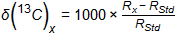
Isotopic ratios are expressed using the delta notation (δ), and the same formula is used regardless of the isotope being determined, although the international standards used are different for the different isotopes (see Section C.9, Table C-2). The δ notation is expressed in the following manner, shown for carbon-13:
Rx corresponds to the ratio of the intensity of the heavy to light isotope in the sample and in the case of RStd, it is the ratio of the heavy to light isotope in the international standard. In the case of carbon, the species actually measured by the IRMS are mass 45 and 44 which correspond to the masses of the 13CO2 and the 12CO2 produced by combustion of the sample. For other isotopes, the appropriate species are again measured and compared to the appropriate standards for each isotope.
Table C-2 presents the reference standards for some of the most commonly applied stable isotopes.
|
Element |
Isotope of interest |
Ratio measured |
Reference standard |
Isotopic ratio |
|---|---|---|---|---|
|
Hydrogen |
2H |
2H/1H |
Vienna Standard Mean Ocean Water (VSMOW) |
1.558 x 10⁻⁴ |
|
Carbon |
13C |
13C/12C |
Vienna Pee Dee Belemnite (VPDB) |
1.118 x 10⁻² |
|
Nitrogen |
15N |
15N/14N |
N2in air |
3.676 x 10⁻³ |
|
Oxygen |
18O |
18O/16O |
VSMOW |
2.005 x 10⁻³ |
|
VPDB |
2.065 x 10⁻³ |
|||
|
17O |
17O/16O |
VSMOW |
3.799 x 10⁻⁴ |
|
|
Sulfur |
34S |
34S/32S |
Vienna Canyon Diablo Troilite (VCDT) |
4.416 x 10⁻² |
|
Chlorine |
37Cl |
37Cl/35Cl |
Standard Mean Ocean Chlorine (SMOC) |
3.196 x 10⁻¹ |
Elements have multiple naturally occurring isotopes. This condition is reflected in the atomic masses of the elements as presented in the periodic table. For example, the most common isotope of carbon is carbon-12 (6 protons, 6 neutrons, or atomic weight of 12.0) but the atomic mass of carbon is 12.011, reflecting the weighted average of 98.9% carbon-12 and 1.1% carbon-13. This small percentage of carbon-13 may then be fractionated between specific compounds in a system (for instance, the degradation intermediate product is slightly ‘lighter’ in carbon-13, and the parent compound is slightly ‘heavier’), but the overall abundance of the isotopes is not impacted.
The natural abundance of the stable isotopes that are of environmental interest are shown in Table C-3. It is important to notice in this table that the heavier isotope is always present in lower abundance than the lighter isotope.
|
Element |
Isotope of Interest (second most abundant stable isotope) |
Ratio measured |
|---|---|---|
|
Hydrogen |
1H/2H |
99.9885/0.0115 |
|
Carbon |
12C/13C |
98.93/1.07 |
|
Nitrogen |
14N/15N |
99.63/0.37 |
|
Oxygen |
16O/18O |
99.759/0.037 |
|
Sulfur |
32S/34S |
94.93/4.29 |
|
Chlorine |
35Cl/37Cl |
75.78/24.22 |
Many common environmental contaminants are derived from crude oil or other fossil fuel sources. Fossil fuels are originally sourced from living organic materials, such as higher plants, phytoplankton, and bacteria. Most of these living systems are photosynthetic systems, meaning that they derive their carbon from the CO2 in the atmosphere by the process of photosynthesis and the hydrogen from groundwater. During the process of photosynthesis the lighter isotope is typically incorporated at a faster rate than the heavier isotope; this process is known as isotopic fractionation.
As a result of different plant types and phytoplankton having different photosynthetic cycles, the extent of fractionation will vary for different species. In living systems, the isotopic composition of a plant or algae can be used to obtain information on the actual photosynthetic cycle. However by the time all this material has accumulated in a sedimentary environment, been buried, and been converted into a fossil fuel, much of the unique isotope signature is lost due to the heterogeneous mixture of organic matter deposited. Despite this loss, crude oils derived from different source materials will have different isotopic signatures, which means individual compounds that are manufactured industrially will often have different isotopic signatures if derived from different feedstocks.
The δ values are an expression of the difference in the isotope ratio of the sample relative to the appropriate international standard, for example a compound that has a carbon isotope value of -25 per mil and is depleted by 25 parts per thousand in the heavier isotope relative to the isotopic composition of the standard. Note that for two samples that are (as an example) -20 and -30 per mil, one can say that the -20 sample is isotopically heavier than the -30 per mil sample. This is sometimes confusing since these are negative numbers. However, the key is to remember that the numbers are reflecting the heavier isotope content of the particular sample being characterized
The majority of environmental hydrocarbon and chlorohydrocarbon samples will have negative isotope ratios. The values for isotopic fractionation at sites are generally isotopically light (negative) compared to the standards due to the selection of specific standards. The carbon standard consists of carbonate, or inorganic carbon, which tends to be isotopically heavy compared to the organic carbon compounds of interest at environmental sites.
The stable isotope compositions of individual compounds can provide two basic types of information in environmental studies: source discrimination (or correlation), and the extent of biodegradation. Source discrimination or apportionment of mixed sources is dependent on sources that are isotopically distinct, due to differing production processes and degree of source degradation. The Rayleigh equation is used to relate degradation-induced decreases in concentrations directly to concomitant changes in bulk (average over the whole compound) isotope ratios.
The most commonly used form of the Rayleigh equation used in environmental studies is shown below:

where:
δ13C at t=0 is the carbon isotopic ratio of the original material (known or estimated)
δ13C at t is the isotopic fractionation measured at the present time (measured during the study)
ε is the enrichment factor (determined in laboratory or microcosmA sample that is regarded as a small but representative portion of something larger. In environmental studies microcosm are typically small samples of soil, sediment, or water incubated in enclosed containers under laboratory conditions. studies)
ln F is the natural logarithm of the remaining concentration of the contaminant
The value of the enrichment factor is needed to calculate the degree of degradation. The isotopic enrichment factor will vary for each compound depending on the microorganisms present and the site conditions. This factor may be measured in microcosm studies, which generate a value for the site organisms under site conditions, or potentially estimated based on a knowledge of organisms present at the site and enrichment factors measured in pure cultures of the organisms.
The extent of in situ transformation, or degradation, may therefore be inferred from measured isotope ratios in field samples, provided that an appropriate enrichment factor (bulk) is known. This bulk value, however, is usually valid for a specific compound and for specific degradation conditions. In other words, enrichment factors that are generally determined from laboratory microcosm studies must be determined for each strain of bacteria thought to be active at a particular site. Because of the time required for microcosm experiments, or the absence of pure cultures, a direct comparison of bulk values for different compounds and for different types of reactions is often not possible.
The enrichment factor is an indication of the degree of isotopic fraction between the parent and intermediate compound during a specific degradation reaction, and it is derived from the fractionation factor α through the relationship ε=1000 (α-1). The factor α reflects the ratio of the rate constants for the heavy/light isotopes. In other words, the different rates at which these species react reflects the extent of changes expected in the isotopic composition of a particular compound during its degradation.
Application of the Rayleigh equation to determine the remaining contaminant from the bulk isotopic fractionation requires the value of the enrichment factors. Different types of bacteria degrading the same compound under different conditions may have different enrichment factors. Additionally, abiotic processes can also cause isotopic shifts.
Enrichment factors are fundamentally a kinetic parameter. Fractionation in degradation reactions results from a slight difference in the energy required to break a bond between two light atoms versus the energy required to break the bond between two atoms of that same type but with one atom being heavy. This relationship is shown in Figure C-1.
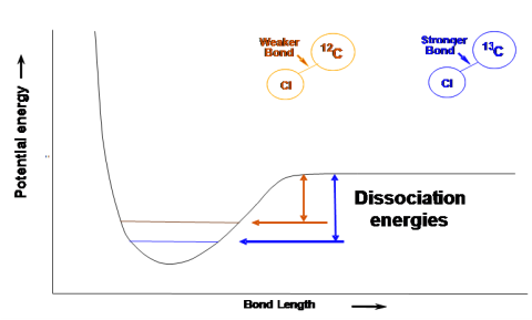
Figure C-1. Schematic indicating the difference in bond dissociation energies that is the origin of isotopic fractionation.
Source: Microseeps, Inc. Used with permission.
When the enrichment factors describe biodegradation, they are a function not just of the small difference in the bond energy portrayed in Figure C-1 but also of the microbial ecology, the strains of bacteria involved, the mass transfer limitations across the cell membrane (see Appendix D, Microbiology FAQ) for the contaminant, the enzymesAny of numerous proteins or conjugated proteins produced by living organisms and facilitating biochemical reactions (based on USEPA 2004a). involved, the availability of contaminant and the toxicity of both the reactants and products in regards to the microbes responsible for the transformation. Thus for biodegradation, enrichment factors are site specific. Further, they are often different at different points in the plume and over the life cycle of the plume.
Studies have shown the mechanism of MTBE biodegradation can be discerned by plotting δ2H vs. δ13C of MTBE, as shown in Figure C-2 (Zwank et al. 2005).
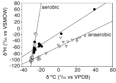
Figure C-2. Graph of δ2H versus δ13C of MTBE. Data points labeled (○) for aerobic biodegradation in a laboratory experiment (Gray et al. 2002); (●) for anaerobic biodegradation at field sites (Kuder et al 2002); (▽) field data reported in Zwank et al. (2005).
Source: Reprinted with permission from Zwank, L., M. Berg, M. Elsner, T.C. Schmidt, R.P. Schwartzenbach, and S.B. Haderlein. 2005. New evaluation scheme for two-dimensional isotope analysis to decipher biodegradation processes: Application to groundwater contamination by MTBE. Environmental Science & Technology 39:1018-1029. Copyright 2005 American Chemical Society.
The slope of the line is the ratio of the enrichment factors εH/εC. Since the data available to that point indicated that anaerobic processes were marked low εH and high εC whereas aerobic processes had higher εH and lower εC, a plot such as that presented in Figure C-2 could be used to discern the biodegradation mechanism.
However, new data has become available (Rosell et al. 2012) that does not fit this model. As of this writing, that data has only been available for several months and the scientific community is still weighing its implications. Future studies may clarify this result. Regardless, at this point two conclusions can be made:
In summary, while exact interpretations are in flux, for some microbes biodegradation of MTBE leads to isotopic enrichment, while biodegradation by other microbes does not lead to enrichment. Observation of enrichment at one site is evidence of biodegradation at that site. Other microbes may be degrading MTBE at a second site and those microbes may not be isotopically enriching the MTBE, so the lack of enrichment at that second site is not conclusive evidence that there is no biodegradation at the second site.
One subset of abiotic remediation is called biogeochemical transformation. This name recognizes the importance of biology and geochemistry in a remediation that relies upon abiotic reactions and is often passive. ESTCP maintains a project on this subject (ER-201124) and held a workshop in February 2008 that issued a report (ESTCP 2008) discussing these transformations in detail. Because the carbon enrichment factors for this process are of a larger magnitude than those of microbial mediated reductive dechlorination, the use of CSIA to distinguish biogeochemical transformation from reductive dechlorination is being pursued (Liang et al. 2007). Similarly, the carbon enrichment factor for the biogeochemical transformation of 1,2-dibromoethane (ethylene dibromide or EDB) is also of a much larger magnitude than the microbial process (USEPA 2008b).
Stable isotopes are useful for source discrimination and for determining the extent of natural attenuation.
Stable isotopes can be a powerful tool for discrimination of multiple sources of a compound. Determination of multiple isotopes (C and H or C and Cl) present in the contaminant can strengthen the evidence for source apportionment. This approach may be limited if the compound of interest from different sources are isotopically similar. For relatively small molecules (typically less that 10 C atoms) it is necessary to establish whether any degradation has occurred – either microbial or abiotic – since this degradation impacts the resulting isotopic composition. Thus it must be established that isotopic differences in these smaller molecules does not result from attenuation processes before concluding that they are coming from different sources.
However, in the case of larger molecules, the use of stable isotopes for the purpose of source discrimination is somewhat easier than with smaller molecules. A larger number of carbon atoms in molecules will cause a smaller, or no, observable fractionation because of an effect known as “internal dilution.” This effect reduces the measurable fractionation in biodegradation of larger molecules such as pesticides. This result implies that differences in the δ13C of pesticides are most likely due to differences in the undegraded pesticides, so material from source A can more readily be distinguished from material from source B, even if significant degradation of either or both sources occurred. Thus, carbon CSIA of pesticides is ideal for forensic applications. Additionally, since chlorinated pesticides have many chlorine atoms in each pesticide molecule, CSIA of chlorine is also ideal for forensic applications of pesticides by the same reasoning. This method has been used by Aeppli et al. 2010.
For many years, determination of natural attenuation has been determined through time-consuming laboratory microcosm studies. With the introduction of GC-IRMS and its ability to determine isotopic compositions of individual compounds, isotopic enrichment of individual compounds has become a powerful tool to determine the onset and extent of natural attenuation. Ranges of source signatures for unaltered groundwater contaminants are fairly well established and compounds that are isotopically heavier than these source signatures can be assigned as being degraded. Use of two or even three isotopes within the same compound provides an even more powerful approach.
Semi-quantitative estimates of the extent of degradation can be obtained through the use of a simplistic form of the Rayleigh equation which equates changes in isotopic composition with concentration changes. More recent efforts have been aimed at incorporating isotope data into flow transport models to provide a more realistic model of changes in isotopic and concentration data over time at specific sites.
Isotopic fractionation provides definitive evidence of degradation of compounds. As mentioned above, isotopic fractionation is used to assess source discrimination and natural attenuation at environmental sites. Stable isotope fractionation data are only useful in the context of a well-developed conceptual site model.
Many of the source discrimination studies involve contaminated groundwater plumes. While some guidelines have been provided in a recent USEPA publication (USEPA 2008a), ideally a good coverage over the complete plume is desired, including the margins as well as the central part of the plume. In many studies, cost and budgetary restraints do not permit large numbers of samples to be collected and analyzed, but as a minimum collect at least 6-10 samples over the plume.
Once samples have been collected and concentrations determined, those samples that are suitable for CSIA can be determined. Initially carbon isotopes should be determined and evaluated in the context of the overall problem being investigated. At that time, a decision can be made as to whether additional isotopes (such as H and Cl) should be determined. In many cases, the two or three isotope approach can be more beneficial than simply using one isotope for source differentiation or evaluation of natural attenuation.
Interpretation of environmental CSIA applications include source correlations; source isotopic signatures; degree of biodegradation (and impact on source isotopic signature); travel distance, hydrogeologic factors, potential for degradation between sources and the site of interest; and natural attenuation.
Several steps are involved when using the stable isotopes for correlation purposes. First, establish that no biodegradation has occurred at the site that may have affected the stable isotope composition of the contaminant of interest. This step can normally be established through the presence of degradation products such as TBA or cis-1,2-DCE. Once this has been established, the isotope ratios can be evaluated in terms of source relationships. Whether samples are related to each other depends to some extent on the precision of the analytical measurements. It is possible to determine the stable carbon isotope compositions of individual groundwater contaminants with a precision of +/- 0.3 per mil. Thus, if a group of samples in a groundwater plume all fall within a range of +/-1 per mil then they may all come from the same source and they are probably related. However, if some samples have isotope ratios that differ by 1.5 per mil or more, and there is no degradation, then those samples may come from a different source.
If there are two or more sources for the plume, then it is possible that the contaminant from both sources may have the same or similar isotopic compositions. In such a situation, it may not be possible to conclusively establish the source of the contaminants in the groundwater. The isotopes will not resolve the sources in every case, but in the situations where isotopic analysis does not provide a solution, none of the other techniques commonly used in these types of problems will provide a solution either. The use of the H and or Cl isotopes may resolve this problem if the concentrations are sufficient to determine the additional isotopes.
Stable isotopes cannot be used to determine the manufacturer of a specific contaminant. Variations in feedstocks, manufacturing conditions, mixing of products from different plants, and many other variables make this an impossibility. When using CSIA, the term “source” is referring to point of release—not the manufacturer of origin.
Biodegradation affects the isotopic signature of the compound of interest. The extent of isotopic enrichment primarily depends upon the compound, mechanism of degradation, and environmental conditions. Changes in isotopic signatures resulting from biodegradation must be recognized or else samples thought to be coming from different sources may simply differ as a result of the degradation process.
Other factors that may affect the source signature of a particular compound may include adsorption, evaporation, and remediation processes such as soil vapor extraction, or partitioning between various phases. However, for most of these physical processes the extent of isotopic fractionation is relatively small (~1 per mil or less) and much smaller than shifts associated with biodegradation.
For most of the common groundwater contaminants ranges of isotopic signatures for unaltered or nondegraded compounds have been clearly established and are summarized in Figure C-3. As the compounds degrade they become isotopically heavier or enriched as a result of preferential cleavage of 12C-12C bonds, leaving the residual substrateAny substance that is acted upon by an enzyme. becoming enriched in the heavier 13C isotope. If these values are heavier than the source signatures by at least 2 or 3 per mil, a high level of confidence exists for contaminant degradation. Certain limitations are associated with these interpretations are summarized below.
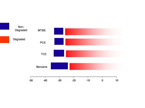
Figure C-3. Comparison between the isotopic compositions of non-degraded versus corresponding degraded components.
Source:Data obtained from papers cited in Philp, R. P. and Jardé, E. (2006). Application of Stable and Radioisotopes in Environmental Forensics. In: Introduction to Environmental Forensics (Murphy and Morrison, Eds. 2007).
In reality, the situation may be far more complex than simply comparing the isotopic composition of the final degradation product, since the isotopic ratios and parent and degradation product are constantly changing. If compound A is simply degrading to compound B, (for example, MTBE to TBA) then the initial TBA will be isotopically light and the MTBE relatively heavy. As the reaction progresses the TBA that is formed continues to become heavier, since the precursor MTBE is also becoming heavier and at the end of the reaction (assuming no TBA has been lost), then the TBA will ultimately have the same isotopic composition as the original MTBE.
In a more complex degradation sequence, for example PCE degrading to TCE, TCE may initially degrade to cis-1,2-DCE. In this case, initially the TCE will be isotopically light but, as it starts to degrade, it will become heavier. At the same time, TCE will also be diluted by more TCE being produced from degradation of the PCE. This is a far more complex situation, but at the end, if all the PCE is totally converted to ethane, then the ethane will have the same isotopic composition as the original PCE. Reactive fate and transport models are currently being developed to take these multiple production and degradation processes into consideration.
CSIA is subject to several limitations.
Reports at a number of sites indicate that no isotope signature of biodegradation was detected even when standard site evaluation criteria were suggestive of degradation. Elsewhere, isotope enrichment was observed, but poor correlation of isotope ratios and concentration attenuation was apparent. While it is possible that attenuation at those sites was primarily due to dispersion, other factors could lead to a false negative interpretation of CSIA. The following general situations regarding potential false negatives are applicable to all common groundwater contaminants.
False positive scenarios are not likely. Non-degradative attenuation pathways under specific hydrological conditions can result in measurable isotope effects. In the studied scenarios, volatilization, air sparging, and SVE resulted in minor carbon isotope effects only. Another interference is a growing number of in situ applications using stable isotope-labeled MTBE and TBA (such as the Bio-Sep® technology). Labeled substrates migrate into groundwater and mimic biodegradation signatures when studied by CSIA (13C labeled MTBE or TBA) or interfere with the instrumental performance of CSIA (any 2H-labeled VOC compounds will potentially interfere with measuring d2H of MTBE). Site managers should take special care to avoid false conclusions if CSIA and stable isotope-label technique are scheduled for the site assessment.
It is sometimes assumed that the isotopic compositions of certain groundwater contaminants can be used to relate these contaminants to a specific manufacturer. This assumption is based on studies published in the early 1990’s in which samples of PCE from different manufacturers were analyzed and led to specific manufacturers. Subsequent research has proven that isotopic analyses cannot reliably relate contaminants to manufacturers. Feedstocks vary on a frequent basis, processes change, and products are fungible. All of these variables and many others render it virtually impossible to associate a certain isotope value with a particular manufacturer.
However, correlations do exist between the suspected release point of a contaminant and samples in the plume. Once it has been established the contaminant is not degraded, then the correlations can be attempted (if possible using two or more isotopes).
Aeppli C., Holmstrand, P. Andersson, and O. Gustafsson. 2010 "Direct Compound-Specific Stable Chlorine Isotope Analysis of Organic Compounds with Quadrupole GC/MS Using Standard Isotope Bracketing." Anal. Chem. 82 (1): 420-426.
Beneteau, K. M., Aravena, R. and Frape, S. K. 1999. "Isotopic characterization of chlorinated solvents-laboratory and field results." Organic Geochemistry 30:739-753.
Coplen,T.B., J. K. Böhlke, P. De Bièvre, T. Ding, N. E. Holden, J. A. Hopple, H. R. Krouse, A. Lamberty, H. S. Peiser, K. Révész, S. E. Rieder, K. J. R. Rosman, E. Roth, P. D. P. Taylor, R. D. Vocke, JR.8 and Y. K. Xiao. 2002. "Isotope-Abundance Variations of Selected Elements (IUPAC Technical Report)." Pure and Applied Chemistry 74 (10):1987-2017.
ESTCP ER-201124. http://www.serdp.org/Program-Areas/Environmental-Restoration/Contaminated-Groundwater/Persistent-Contamination/ER-201124/ER-201124/(language)/eng-US
ESTCP 2008. Workshop on In Situ Biogeochemical Transformation of Chlorinated Solvents. Feb. 2008.
Gray, J. R., G. Lacrampe-Couloume, D. Gandhi, K. M. Scow, R. D. Wilson, D. M. Mackay and B. Sherwood Lollar. 2002. “Carbon and hydrogen isotopic fractionation during biodegradation of methyl tert-butyl ether.” Environmental Science &Technology 36:1931-1938.
Jin, B., C. Laskov, M. Rolle, and S.B. Haderlein. 2011. “Chlorine Isotope Analysis of Organic Contaminants Using GCqMS: Method Optimization and Comparison of Different Evaluation Schemes.” Environmental Science & Technology 45:5279-5286.
Liang, X., Y. Dong, T. Kuder, L. R. Krumholz, R. P. Philp and E. C. Butler. 2007. “Distinguishing abiotic and biotic transformation of tetrachloroethylene and trichloroethene by stable carbon isotope fractionation.” Environmental Science & Technology 41 (20): 7094-7100.
Kuder, T.; Philp, R. P.; Kolhatkar, R.; Wilson, J. T.; Allen, J. 2002. “Application of stable carbon and hydrogen isotopic techniques for monitoring biodegradation of MTBE in the field.” In NGWA/API Petroleum Hydrocarbons and Organic Chemicals in GroundWater; American Petroleum Institute.
Murphy, B. L. and R. D. Morrison. 2007. Introduction to Environmental Forensics. Edition 2. Elsevier Science. Philp, R.P and E. Jardé, Chapter 10: "Application of Stable Isotopes and Radio Isotopes in Environmental Forensics."
Rosell, M., R. Gonzalez-Olmos, T. Rohwerder, K. Rusevova, A. Georgi, F.-D. Kopinke, and H.H. Richnow. 2012. "Critical evaluation of 2D-CSIA scheme for distinguishing fuel oxygenate degradation reaction mechanisms." Environmental Science &Technology 46: 4757-4766.
Rosman, K.J.R. and P.D.P Taylor.1998. Isotopic compositions of the elements (Technical Report). Pure & Applied Chemistry 70 (1):217-235.
Santrock J, Studley S.A. and Hayes J.M. 1985. “Isotopic analyses based on the mass spectrum of carbon dioxide”. Anal. Chem. 57:14444-1448.
Sessions A.L., T.W. Burgoyne, and J. M. Hayes. 2001. "Correction of H3+ Contributions in Hydrogen Isotope Ratio Monitoring Mass Spectrometry." Analytical Chemistry 73: 192-199.
Shouakar-Stash, O., Drimmie, R.J., Zhang, M. and Frape, S.K. 2006. “Compound Specific Chlorine Isotopic Ratios of TCE, PCE and DCE isomers by direct injection using CF-IRMS.” Applied Geochemistry 21:766-781.
USEPA 2008a. A Guide for assessing biodegradation and source identification of organic ground water contaminants using compound specific isotope analysis (CSIA)Analyzes the relative abundance of various stable isotopes (e.g., ¹³C:¹²C, ²H:¹H). Degradation processes can cause shifts in the relative abundance of stable isotopes of the contaminant; changes in isotopic ratios can be measured.. EPA 600/R-08/148.
USEPA. 2008b. Natural Attenuation of the Lead Scavengers 1,2-Dibromoethane (EDB) and 1,2-Dichloroethane (1,2-DCA) at Motor Fuel Release Sites and Implications for Risk Management. 600/R-08/107.
Zwank, L., M. Berg, M. Elsner, T.C. Schmidt, R.P. Schwartzenbach, and S.B. Haderlein. 2005. "New evaluation scheme for two-dimensional isotope analysis to decipher biodegradation processes: Application to groundwater contamination by MTBE." Environmental Science & Technology 39:1018-1029.